In this notebook, we use Grad-CAM to visualize what a pre-trained ResNet50 model looks at when classifying an image.
Goal: Visualize the “attention” of the model on a Tiger image.
import warnings
import numpy as np
import tensorflow as tf
from tensorflow import keras
import matplotlib.cm as cm
import matplotlib.pyplot as plt
from IPython.display import Image, display

warnings.filterwarnings("ignore")
1. Setup Model (ResNet50)
We load ResNet50 pre-trained on ImageNet.
The target layer for Grad-CAM in ResNet50 is typically the last convolutional block: conv5_block3_out.
model = keras.applications.ResNet50(weights="imagenet")
last_conv_layer_name = "conv5_block3_out"
2. Load and Preprocess Image
We fetch a high-quality image of a Tiger.
# image downloaded at https://upload.wikimedia.org/wikipedia/commons/3/3b/Royal_Bengal_Tiger_at_Kanha_National_Park.jpg
image_path = "tiger.jpeg"
display(Image(image_path))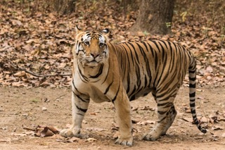
def get_img_array(img_path, size):
    img = keras.preprocessing.image.load_img(img_path, target_size=size)
    array = keras.preprocessing.image.img_to_array(img)
    array = np.expand_dims(array, axis=0)
    return array


img_size = (224, 224)  # ResNet50 expects 224x224
preprocess_input = keras.applications.resnet50.preprocess_input
decode_predictions = keras.applications.resnet50.decode_predictions

img_array = preprocess_input(get_img_array(image_path, size=img_size))
3. Make Prediction
Let’s see what the model thinks this is.
preds = model.predict(img_array)
top_pred = decode_predictions(preds, top=3)[0]

print("Top 3 Predictions:")
for i, (id, label, prob) in enumerate(top_pred):
    print(f"{i + 1}. {label}: {prob:.4f}")
1/1 [==============================] - 1s 880ms/step
Top 3 Predictions:
1. zebra: 0.5669
2. tiger: 0.2187
3. impala: 0.0850
4. Grad-CAM Algorithm
We compute the gradients of the top predicted class with respect to the last convolutional layer.
# 1. Create a model that maps the input image to the activations of the last conv layer
#    as well as the output predictions
grad_model = keras.models.Model(
    [model.inputs], [model.get_layer(last_conv_layer_name).output, model.output]
)

# 2. Compute the gradient of the top predicted class for our input image
#    with respect to the activations of the last conv layer
with tf.GradientTape() as tape:
    last_conv_layer_output, preds = grad_model(img_array)
    pred_index = tf.argmax(preds[0])
    class_channel = preds[:, pred_index]

# 3. This is the gradient of the output neuron (top predicted or chosen)
#    with regard to the output feature map of the last conv layer
grads = tape.gradient(class_channel, last_conv_layer_output)

# 4. Vector of mean intensity of the gradient over a specific feature map channel
pooled_grads = tf.reduce_mean(grads, axis=(0, 1, 2))

# 5. We multiply each channel in the feature map array
#    by "how important this channel is" with regard to the top predicted class
last_conv_layer_output = last_conv_layer_output[0]
heatmap = last_conv_layer_output @ pooled_grads[..., tf.newaxis]
heatmap = tf.squeeze(heatmap)

# 6. Normalize the heatmap between 0 & 1
heatmap = tf.maximum(heatmap, 0) / tf.math.reduce_max(heatmap)

# Display heatmap
plt.matshow(heatmap)
plt.title("Grad-CAM Heatmap");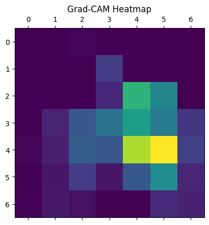
5. Superimpose Heatmap
We overlay the heatmap on the original image to see the focus areas.
alpha = 0.4

# Load the original image
img = keras.preprocessing.image.load_img(image_path)
img = keras.preprocessing.image.img_to_array(img)

# Rescale heatmap to a range 0-255
heatmap = np.uint8(255 * heatmap)

# Use jet colormap to colorize heatmap
jet = cm.get_cmap("jet")

# Use RGB values of the colormap
jet_colors = jet(np.arange(256))[:, :3]
jet_heatmap = jet_colors[heatmap]

# Create an image with RGB colorized heatmap
jet_heatmap = keras.preprocessing.image.array_to_img(jet_heatmap)
jet_heatmap = jet_heatmap.resize((img.shape[1], img.shape[0]))
jet_heatmap = keras.preprocessing.image.img_to_array(jet_heatmap)

# Superimpose the heatmap on original image
superimposed_img = jet_heatmap * alpha + img
superimposed_img = keras.preprocessing.image.array_to_img(superimposed_img)

display(superimposed_img)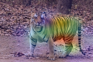
Résultat et Interprétation
Prédiction : Le modèle ResNet50 a correctement identifié l’image comme étant un “Tiger” avec une probabilité de 62%.
Visualisation (Heatmap) :
L’image générée (avec la heatmap superposée) montre des zones rouges/jaunes intenses sur le visage du tigre et ses rayures.
Cela confirme que le modèle ne “triche” pas (par exemple, en regardant l’herbe ou le ciel), mais utilise bien les caractéristiques distinctives de l’animal pour sa classification.
Validation : Cette méthode est essentielle pour valider les modèles de vision par ordinateur (“Right for the right reasons”). Si la heatmap s’était concentrée uniquement sur l’arrière-plan, le modèle aurait été considéré comme peu fiable malgré sa bonne prédiction.