Main Concept
IsoMap transforms the original high-dimensional data by attempting to preserve geodesic distances between points rather than Euclidean distances.
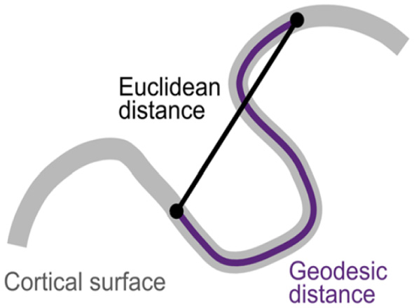
Euclidean vs. Geodesic distance
The geodesic distance is approximated by finding the shortest path between points along a neighborhood graph. After applying IsoMap, data points receive new coordinates in a lower-dimensional space where the Euclidean distances between points approximate the original geodesic distances. This helps to “unfold” nonlinear manifolds - imagine straightening out a rolled-up piece of paper while preserving the distances along its surface.
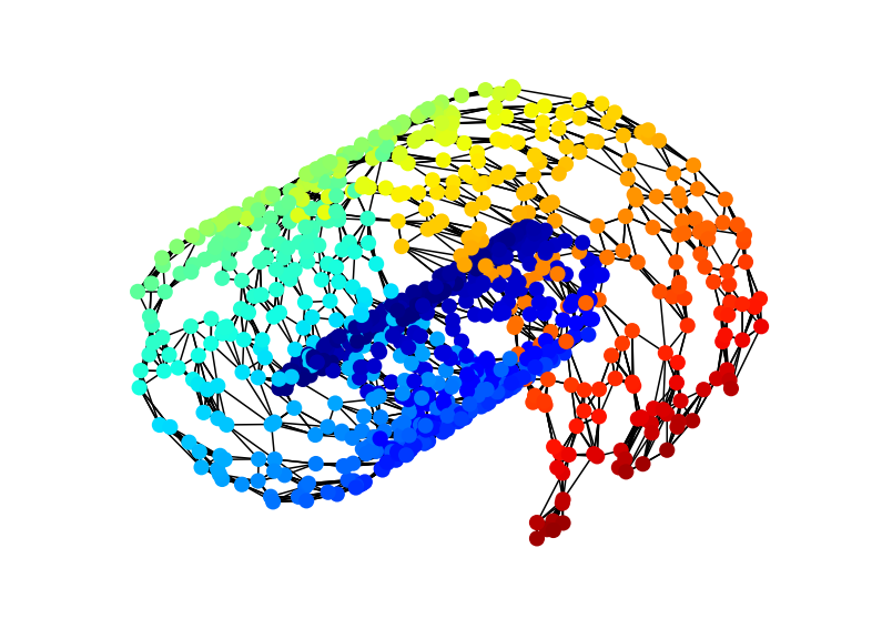
Geodesic neighboorhood on a 3D Swiss-roll
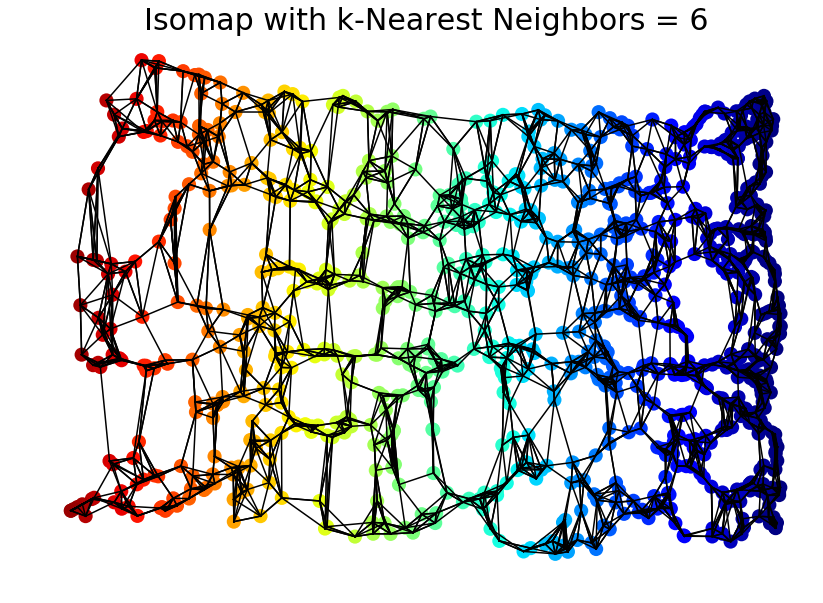
Unfolded 3D Swiss-roll with original geodesic graph
Theoretical Aspect
The optimization problem in IsoMap can be formulated as:
Where:
- is the geodesic distance between points i and j in the original space
- and are the coordinates of points i and j in the new low-dimensional space
- is the Euclidean distance between points in the new space
The key variables being optimized are the coordinates Y of all points in the lower-dimensional space.
Solution Methodology
IsoMap follows these main steps:
- Construct neighborhood graph by connecting each point to its k nearest neighbors or all points within ε distance
- Compute geodesic distances between all pairs of points using Floyd-Warshall or Dijkstra’s algorithm
- Apply Classical MDS to the geodesic distance matrix:
- Center the distance matrix
- Compute eigendecomposition of the centered matrix
- Project onto top eigenvectors to get final coordinates
The solution leverages the fact that Classical MDS has a closed-form solution through eigendecomposition, making it computationally efficient.
Global Optimality
The IsoMap solution has interesting optimality properties:
- The eigendecomposition step provides a globally optimal solution to the MDS step
- However, the overall method is not guaranteed to find a global optimum of the true manifold learning problem because:
- The neighborhood graph construction is a discrete approximation
- The geodesic distance estimation depends on the graph structure and may not perfectly capture the true manifold distances
- The method assumes the manifold is isometric to a convex subset of Euclidean space
Key limitations include:
- Sensitivity to the choice of neighborhood size/radius
- Potential “short-circuiting” if the neighborhood graph connects distant parts of the manifold
- Poor performance when the manifold is not approximately isometric to a convex subset of Euclidean space
- Computational complexity of for n data points, making it challenging for large datasets
Conclusion
Despite these limitations, IsoMap often performs well in practice when its assumptions are reasonably satisfied and has become a fundamental algorithm in the manifold learning toolkit.